bcam.indar.ema.StablePoles

class bcam.indar.ema.StablePoles(model, max_order, *, radius: float | None = None, min_scale: int = -10)

Stabilization diagram.

This class helps to identify stable poles across different orders of spectral estimation. Since the algorithm tends to find more stable poles than really exist, post-processing is recommended.

Parameters:

model: BaseEstimator

Model for spectral estimation. The class is designed to work with SuperResolution, but it also accepts custom models as long as they behave similarly to SuperResolution.

max_order: int

Maximum order of the exponential sum. Recall that complex poles come in conjugate pairs, so they count as two.

radius: float, optional

Maximum threshold for adding poles to a cluster. If None, the radius is set to \(d(0, 0.5)\); see Notes for details.

min_scale: int, default=-10

Lowest amplitude level for clustering; see Notes for details.

Attributes:

clusters_list of dict

List of clusters of poles. Each cluster is a dictionary where the keys are the orders of the poles and the values are the poles themselves. The clusters are sorted by decreasing number of poles. If two clusters have the same size, then they are sorted increasing standard deviation of the poles.

clusters_amps_list of dict

List of clusters of amplitudes corresponding to the poles in clusters_. Only the norm of the amplitudes is stored.

Methods

clusters_stats()	Get statistics of the clusters.
fit(y)	Fit exponential sums and find clusters.
plot_clusters([clusters, ax])	Plot clusters of poles.
plot_poles(level[, ax])	Plot poles at a given level.

Notes

The clustering algorithm first groups poles by the norm of the amplitudes, so if \(A\) is the largest amplitude accross all orders, then the levels are defined as the (non-disjoint) intervals \([A/2^{l+3}, A/2^l]\) for \(l = 0, 1, \ldots\). Then, the algorithm sets all the poles at order max_order as seeds for clustering. At each step, starting from the highest order and downwards, all the poles at the given order — and within the same amplitude level — are added to their closest cluster if they are within the given radius from it; unassigned poles are set as seeds for new clusters. Finally, clusters with less than 25% of the total number of orders are discarded.

To measure the distance between poles, we use the following metric:

\[d(p, q) = \sqrt{\frac{1}{n}\sum_{k=0}^{n-1} |p^k - q^k|^2}\]

where \(n\) is the length of the signal to be approximated. This distance is motivated by the fact that the poles are used to construct exponential sums, so it is more meaningful to measure the distance between poles in terms of their effect on the exponential sum rather than their Euclidean distance in the complex plane.

Examples

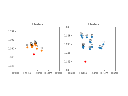
We generate a signal with two natural frequencies, and use the stabilization diagram to identify them. The maximum order we fit is 40, which roughly corresponds to 20 pairs of poles (ignoring real ones).

>>> import numpy as np
>>> import matplotlib.pyplot as plt
>>> from bcam.indar import ema
>>> # Set the parameters of the exponential sum.
>>> freqs = np.array([-0.8 + 1j*20.3, -1.3 + 1j*42.5])
>>> amps = np.array([0.5+1j*0.8, 0.3-1j*0.1])
>>> # Set the sampling parameters.
>>> dt = 0.02
>>> t = np.arange(0, 100) * dt
>>> # Generate the signal and add noise.
>>> y = np.sum(
...     amps[np.newaxis, :]*np.exp(freqs[np.newaxis, :]*t[:, np.newaxis]),
...     axis=1)
>>> y = np.real(y)
>>> rng = np.random.default_rng(1234)
>>> y += rng.normal(0, 0.05, size=y.shape)
>>> # Define the model for spectral estimation.
>>> model = ema.SuperResolution(
...    rational_fitter={'method': 'AAA'}, fs=1/dt)
>>> # Construct stabilization diagram.
>>> sp = ema.StablePoles(model=model, max_order=40)
>>> sp.fit(y)

The algorithm detects three clusters, we can discard one of them because its number of poles and amplitudes are small. The method StablePoles.plot_clusters() also annotates the order of each pole.

>>> fig, ax = plt.subplots(ncols=2)
>>> sp.plot_clusters(ax=ax[0])
>>> sp.plot_clusters(ax=ax[1])
>>> # Plot true poles in red.
>>> true_poles = np.exp(freqs*dt)
>>> for i, p_ in enumerate(true_poles):
>>>    ax[i].scatter(p_.real, p_.imag, color='red')
>>>    ax[i].legend().remove()
>>> # Zoom in to the clusters.
>>> ax[0].set_xlim(0.9, 0.91)
>>> ax[0].set_ylim(0.385, 0.395)
>>> ax[1].set_xlim(0.64, 0.65)
>>> ax[1].set_ylim(0.73, 0.74)
>>> # Increase spacing between subplots.
>>> plt.subplots_adjust(wspace=0.3)
>>> plt.show()

(png)

clusters_stats()

Get statistics of the clusters.

Returns:

statspandas.DataFrame

DataFrame containing the statistics of the clusters.

Raises:

ValueError

If fit() has not been run.

fit(y: array - like) → StablePoles

Fit exponential sums and find clusters.

Parameters:

yarray-like, shape (n_time_samples, n_channels)

Time series to be approximated by exponential sums.

Returns:

selfStablePoles

plot_clusters(clusters: list[int] | None = None, ax: Axes | None = None)

Plot clusters of poles.

Parameters:

clusterslist of int, optional

List of cluster indices to plot. If None, all clusters are plotted.

axmatplotlib.axes.Axes, optional

Axes to plot on. If None, a new figure and axes are created.

Raises:

ValueError

If fit() has not been run.

plot_poles(level: float, ax: Axes | None = None)

Plot poles at a given level.

Parameters:

levelfloat

Level to plot poles.

axmatplotlib.axes.Axes, optional

Axes to plot on. If None, a new figure and axes are created.

Raises:

ValueError

If fit() has not been run.