Getting Started

The indar package collects tools and methods developed during our research, and it is not intended as a general-purpose package with a fixed high-level workflow. At the moment, it provides methods for Experimental Modal Analysis (EMA) and for solving eigenvalue problems of Delay Differential Equations (DDE) with a single delay.

This example shows a complete EMA workflow using indar.

Tuned Mass Damper

In this example, we will use the core utilities of indar.ema to estimate the modal parameters of a mechanical system. We process data from a simulated hammer test of a Tuned Mass Damper (TMD), where the measured signals are the input force and output accelerations.

We start by loading and inspecting the data, then estimate the system Impulse Response Function (IRF). The IRF is defined for any causal Linear Time-Invariant (LTI) system. For mechanical systems, however, the IRF is an exponential sum, so we can estimate its order and natural frequencies.

Finally, we estimate the mode shapes and compare the identified modal parameters with the true ones.

For this example, we recommend to create an environment with the following dependencies:

• numpy

• pandas

• matplotlib

• scikit-learn

• scipy

• bcam-indar (install with pip install bcam-indar)

We simulate a hammer test of the Tuned Mass Damper (TMD) in the figure below, which is a 2-DoF system.

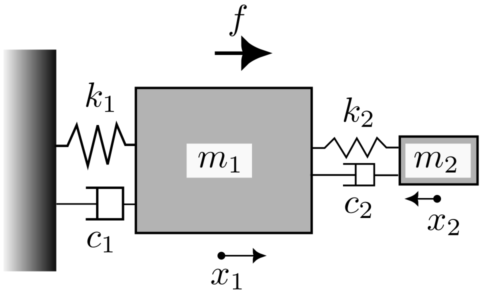
The system is excited at the first mass, and the response is measured at both masses. The equation of motion of the system is

\[\begin{split}\begin{gathered} M\ddot{x} + C\dot{x} + Kx = f \\ M = \begin{bmatrix} m_1 & 0 \\ 0 & m_2 \end{bmatrix},\quad C = \begin{bmatrix} c_1 + c_2 & -c_2 \\ -c_2 & c_2 \end{bmatrix},\quad K = \begin{bmatrix} k_1 + k_2 & -k_2 \\ -k_2 & k_2 \end{bmatrix}, \end{gathered}\end{split}\]

with parameters in the table below.

Mass	Damping	Stiffness
\(m_1 = 1.0\)	\(c_1 = 1.6\)	\(k_1 = 400.0\)
\(m_2 = 0.05\)	\(c_2 = 0.242\)	\(k_2 = 18.14\)

The test is repeated four times with a sampling interval of \(\Delta t = 0.02\), and the number of time samples is 256.

To follow the example along, download the data files 2-dof-system_rep*.csv from this link and save them in a directory called data. Alternatively, execute the following command in your bash terminal:

wget -nv -P data https://raw.githubusercontent.com/CFAA-EHU/bcam-indar/main/docs/source/_documents/2-dof-system_rep{0..3}.csv

To load and inspect the data, execute the following code in your Python environment:

# Import libraries
import os

import numpy as np
import pandas as pd
import matplotlib.pyplot as plt

# Load data
impact = []
response = []
n_rep = 4 # number of repetitions
for rep in range(n_rep):
    file = os.path.join('data', f'2-dof-system_rep{rep}.csv')
    df = pd.read_csv(file, sep=',')
    impact.append(df['impact'].values)
    response.append([df['response_0'].values, df['response_1'].values])
impact = np.array(impact) # shape: (n_rep, 256)
response = np.array(response)  # shape: (n_rep, 2, 256)

dt = 0.02 # sampling interval
ns = impact.shape[-1] # number of time samples
n_in, n_out = 1, 2

# Plot data for the first trial
fig, axs = plt.subplots(ncols=2, sharex=True, figsize=(10, 4))
tt = np.arange(ns)*dt
axs[0].set_title('Impact')
axs[0].plot(tt, impact[0, :])
axs[0].set_xlabel('Time')
axs[0].set_ylabel('Force')

axs[1].set_title('Response')
axs[1].plot(tt, response[0, 0, :], label='mass 1')
axs[1].plot(tt, response[0, 1, :], label='mass 2')
axs[1].set_xlabel('Time')
axs[1].set_ylabel('Acceleration')
axs[1].legend()

fig.tight_layout()
plt.show()

(png)

Impulse Response Function

We will not use the H1 estimator but the class bcam.indar.ema.LTIKernel. The estimator used by this class is based on a time-domain model, which means that the estimation is not affected by leakage, so it can be used with any type of excitation and time-window without introducing bias in the estimation. For example, in case of random excitations, it is not necessary to ensure periodicity. However, its downside is that the estimation takes considerably more time than the H1 estimator.

The class LTIKernel has two parameters, \(\alpha\) and \(\beta\), which control the regularization of the estimation. To choose these parameters we may manually inspect the estimated IRF and choose the one that looks best. However, LTIKernel can be coupled with sklearn.model_selection.GridSearchCV to automatically select the best parameters based on a scoring function.

# Import libraries
from bcam.indar import ema
from sklearn.model_selection import GridSearchCV

# Create model to estimate the IRF
lti_model = ema.LTIKernel(dt=dt, mode='a')

# Define parameters to search in cross-validation
pmts = {
    'alpha': np.array([1e-2, 1.]),
    'beta': 10**np.linspace(0, 2, 8)
}
clf = GridSearchCV(
    lti_model, pmts, cv=n_rep,
    scoring='neg_mean_squared_error',)
r, e = 1, 0 # response (r), input (e)
clf.fit(impact[:, :], response[:, r, :])
# Choose the best model
lti_model = clf.best_estimator_

# Use the best model to estimate the IRF
irf_ = np.zeros((n_out, n_in, ns)) # Shape: (2, 1, 256)
for i in range(n_out):
    # The more repetitions, the better the estimation.
    lti_model.fit(impact, response[:, i, :])
    irf_[i, 0, :] = lti_model.kernel_

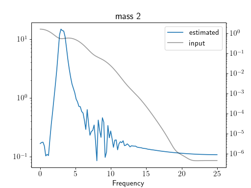
The array irf_ contains the estimated IRF with the best parameters found by cross-validation. If we inspect clf, we will see that the best parameters are \(\alpha = 0.01\) and \(\beta = 7.20\). We now plot the estimated FRF of mass 2 together with the input spectrum. This helps identify the frequency range where low input energy may reduce estimation quality.

fig, ax = plt.subplots()
axt = ax.twinx() # Twin axis to plot the input spectrum

frf_ = np.fft.rfft(irf_, axis=-1)*dt # Compute FRF
ax.set_title('mass 2')
freqs = np.fft.rfftfreq(ns, dt)
ax.plot(
    freqs, np.abs(frf_[r, e]), label='estimated')
axt.plot(
    freqs, np.abs(np.fft.rfft(impact[0, :]))*dt, label='input',
    color='k', alpha=0.4)

ax.set_xlabel('Frequency')
ax.set_yscale('log')
axt.set_yscale('log')
# Combine legends of both axes
lines1, labels1 = ax.get_legend_handles_labels()
lines2, labels2 = axt.get_legend_handles_labels()
ax.legend(lines1 + lines2, labels1 + labels2, loc='upper right')

plt.show()

(png)

Spectral estimation

Because the IRF of a mechanical system is an exponential sum, estimating modal frequencies can be recast as a rational approximation problem. Here we use the AAA algorithm for that step.

We use bcam.indar.ema.StablePoles to construct a stabilization diagram up to order 30 (complex poles appear in conjugate pairs) and then summarize the resulting stable-pole clusters.

# Use AAA as algorithm for rational approximation
sr = ema.SuperResolution(
    fs=1/dt, rational_fitter={'method': 'AAA'})
# Construct stabilization diagram
sp = ema.StablePoles(sr, max_order=30)
sp.fit(irf_[:, 0, :].T)

# Summarize clusters
sp.clusters_stats()

number	pole	pole cv.	amp.	amp. cv.	highest order	lowest order
14	0.913+0.334j	0.0173	20.6	0.0183	30	5
14	-0.0833+0j	0.986	52	0.0384	30	5
14	0.874+0.4j	0.0242	26.5	0.0254	30	5

As expected, the table shows three stable-pole clusters. The first column gives the number of poles per cluster, where each pole comes from a different model order in the stabilization diagram. The table also reports cluster means for poles and amplitude magnitudes, together with their coefficient of variation (cv).

Two clusters correspond to the system’s complex-conjugate mechanical poles. The third approximates the mass-term from the accelerance, which appears as a Dirac delta at time zero. Consistent with that interpretation, the two mechanical clusters have similar amplitudes, while the Dirac-like term has a comparatively large contribution.

The AAA algorithm is fast but not very robust against noise, so we use Vector Fitting (VF) to refine the estimation of the poles.

# Use the poles estimated by AAA as initial poles for VF
sr = ema.SuperResolution(
    order = sr.poles_.count(),
    rational_fitter={
        'method': 'VF',
        'poles': (sr.poles_.real, sr.poles_.cx),
        'niter': 5
    },
    compute_amps=False,
    fs=1/dt)
sr.fit(irf_[:, 0, :].T)

The object sr now contains the refined poles in poles_. At this point we distinguish two groups: mechanical poles and background poles.

Mode shapes

The next step is to estimate mode shapes. To do that, we first estimate IRF amplitudes with bcam.indar.ema.Amplitudes. At this stage, we also impose additional physical constraints, such as Maxwell’s reciprocity.

Inspecting sr.poles_, the first two poles match the mechanical poles identified in the stabilization diagram, while the remaining poles are treated as background poles.

model = ema.Amplitudes(
    mech_poles=sr.poles_.cx[:2], # mechanical poles
    res_poles=(sr.poles_.real, sr.poles_.cx[2:]), # background poles
    fs=1/dt,
    response='a')
model.fit(irf_)

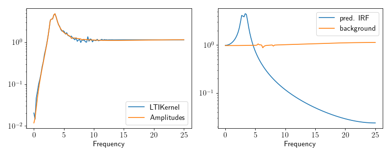
We now compare two FRF estimates for response at mass 1: LTIKernel and Amplitudes. Recall that LTIKernel estimates a general LTI IRF, whereas Amplitudes enforces the exponential-sum structure.

We also plot the two components from Amplitudes: the predicted structural IRF and the background term, which contains noise and the mass-term of the accelerance.

fig, axs = plt.subplots(ncols=2, sharex=True, figsize=(10, 4))

r, e = 0, 0 # response (r), input (e)
freqs = np.fft.rfftfreq(ns, dt)

# Plot the FRF estimated by the classes LTIKernel and Amplitudes
fft_pred = model.predict(np.arange(ns)*dt)
fft_pred = np.fft.rfft(fft_pred, axis=-1)*dt
axs[0].plot(freqs, np.abs(frf_[r, e]), label='LTIKernel')
axs[0].plot(freqs, np.abs(fft_pred[r, e]), label='Amplitudes')
axs[0].set_xlabel('Frequency')
axs[0].set_yscale('log')
axs[0].legend(loc='lower right')

# Plot the predicted IRF and background.
# Since the background contains the mass-term,
# its FRF resembles a constant function.
frf_irf_pred = model.irf_pred(np.arange(ns)*dt)
frf_bckg = model.residual(np.arange(ns)*dt)
frf_irf_pred = np.fft.rfft(frf_irf_pred, axis=-1)*dt
frf_bckg = np.fft.rfft(frf_bckg, axis=-1)*dt
axs[1].plot(freqs, np.abs(frf_irf_pred[r, e]), label='pred. IRF')
axs[1].plot(freqs, np.abs(frf_bckg[r, e]), label='background')
axs[1].set_xlabel('Frequency')
axs[1].set_yscale('log')
axs[1].legend()

fig.tight_layout()
plt.show()

(png)

To estimate mode shapes under proportional damping, we use bcam.indar.ema.RealModes. It applies a global minimizer to match the amplitudes \(A^l_{ij}\) estimated by Amplitudes with the products \(\varphi_{il} \varphi_{jl}\).

tensor_modes = model.tensor_modes_ # These are the amplitudes A^l_{ij}
model_r = ema.RealModes(
    poles=sr.poles_.cx[:2], # mechanical poles
    amps=tensor_modes,
    fs=1/dt,
    ns=ns,
    response='a',
)
model_r.fit(
    options_ncg={'disp': 0, 'gtol': 1e-5}, # Change disp to 1 to see details
)

Because the poles are close, modal coupling can be significant. To refine the result, we drop the assumtion of proportional damping and estimate mode shapes with bcam.indar.ema.ComplexModes.

model_cx = ema.ComplexModes(
    poles=sr.poles_.cx[:2], # mechanical poles
    coords=np.arange(n_out),
    amps=tensor_modes, # These are the amplitudes A^l_{ij}
    fs=1/dt,
    ns=ns,
    response='a'
)
model_cx.fit(
    x0=model_r.modes_, # As initial guess, we use the estimated real mode shapes
    maxiter=100,
    options={'verbose': 0, 'gtol': 1e-5, 'xtol': 1e-6} # Change verbose to 1 or 2 to see details
)

During optimization, ComplexModes may warn that some matrices are not positive definite. These warnings can appear when constraints are temporarily violated and are not always problematic. However, if warnings appear persistently, optimization is likely struggling to find a stable solution.

We then compare FRFs reconstructed with real and complex mode shapes.

fig, axs = plt.subplots(ncols=2, sharex=True, figsize=(10, 4))

e = 0
freqs = np.fft.rfftfreq(ns, dt)

fft_r = model_r.predict(np.arange(ns)*dt)
fft_r = np.fft.rfft(fft_r, axis=-1)*dt
fft_cx = model_cx.predict(np.arange(ns)*dt)
fft_cx = np.fft.rfft(fft_cx, axis=-1)*dt

for r in range(n_out):
    axs[r].set_title(f'response {r}')
    axs[r].plot(freqs, np.abs(fft_r[r, e]), label='RealModes')
    axs[r].plot(freqs, np.abs(fft_cx[r, e]), label='ComplexModes')
    axs[r].set_xlabel('Frequency')
    axs[r].set_yscale('log')

axs[1].legend()
axs[0].set_xlim(0, 10)
axs[0].set_ylim(1e-1, 9)

fig.tight_layout()
plt.show()

(png)

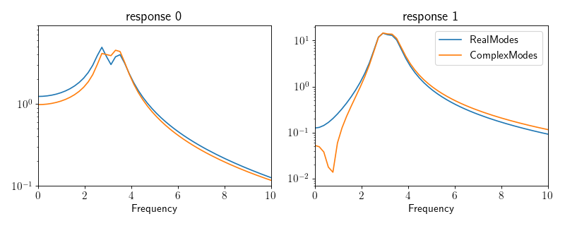
Although both reconstructions are similar, their difference is still clearly visible.

Note

In general, estimating complex mode shapes is challenging. It works well here because only two close modes are involved. If a third complex pole were present at a very different natural frequency, the optimizer would be more likely to stall after many iterations.

When poles are clustered and damping is sufficiently high, convergence becomes more likely. Lack of convergence, however, does not imply that the system has proportional damping.

To assess estimation quality, we compare the FRF reconstructed from complex mode shapes with the true system FRF.

# Compute modal representation of the system.
# The user must introduce the matrices M, C, and K manually before running this code.
mode_shapes, nat_freqs = ema.system_to_modal(M, C, K)
# The mode shapes are returned normalized by mass,
# but we need them in the reduced normalization
mode_shapes = mode_shapes / np.sqrt(np.imag(nat_freqs))
# We compute the amplitudes of the true FRF
amps = ema.mode_to_amps(mode_shapes, n_out=2, n_in=2)

# Compute the true FRF of the system
frf_true = ema.Kernel(nat_freqs, amps)
tt = np.arange(ns)*dt
frf_true = frf_true(tt)
frf_true = np.fft.rfft(frf_true, axis=-1)*dt

fig, axs = plt.subplots(ncols=2, sharex=True, figsize=(10, 4))

freqs = np.fft.rfftfreq(ns, dt)
for r in range(n_out):
    axs[r].set_title(f'response {r}')
    axs[r].plot(freqs, np.abs(frf_true[r, e]), label='true FRF')
    axs[r].plot(freqs, np.abs(fft_cx[r, e]), label=f'estimated FRF')
    axs[r].set_xlabel('Frequency')
    axs[r].set_yscale('log')

axs[1].legend()
axs[0].set_xlim(0, 10)
axs[0].set_ylim(1e-1, 9)

fig.tight_layout()
plt.show()

(png)

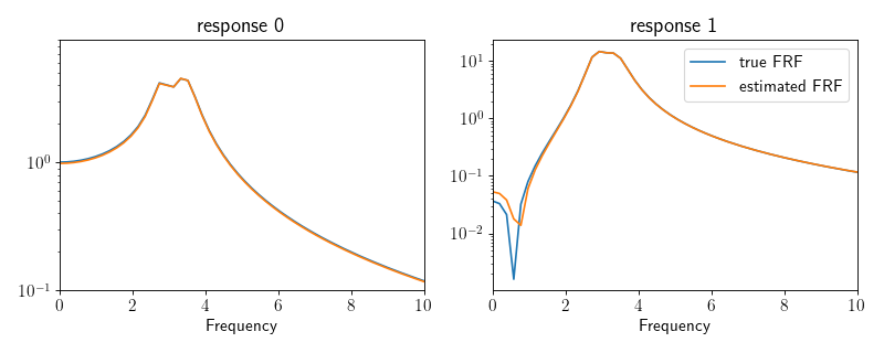
The two FRFs show good agreement. We can then estimate mass, damping, and stiffness matrices with

\[M = \im\big(\varphi \Lambda \varphi^T\big)^{-1}, \quad K = -\im\big(\varphi \Lambda^{-1} \varphi^T\big)^{-1}, \quad\text{and}\quad C = -M\im\big(\varphi \Lambda^2 \varphi^T\big)M,\]

where \(\varphi\) are the mode shapes (real or complex) arranged as an \((n_\mathrm{out} \times \mathrm{dof})\)-matrix.

# Estimated modal parameters
modes_ = model_cx.modes_
poles_ = sr.poles_.cx[:2]
nat_freqs_ = np.log(poles_)/dt

# Estimated mass, damping, and stiffness matrices
M_ = np.imag((modes_*nat_freqs_[np.newaxis, :]) @ modes_.T)
M_ = np.linalg.inv(M_)

K_ = -np.imag((modes_/nat_freqs_[np.newaxis, :]) @ modes_.T)
K_ = np.linalg.inv(K_)

C_ = -np.imag((modes_*nat_freqs_[np.newaxis, :]**2)@modes_.T)
C_ = M_ @ C_ @ M_

Below, we compare the true matrices (left) with the estimated matrices (right).

\[\begin{split}M = \begin{bmatrix}1 & 0 \\ 0 & 0.05\end{bmatrix}, \qquad \hat{M} = \begin{bmatrix}1.021 & 0.0007782 \\ 0.0007782 & 0.05093\end{bmatrix}\end{split}\]

\[\begin{split}C = \begin{bmatrix}1.842 & -0.2424 \\ -0.2424 & 0.2424\end{bmatrix}, \qquad \hat{C} = \begin{bmatrix}1.771 & -0.2542 \\ -0.2542 & 0.2474\end{bmatrix}\end{split}\]

\[\begin{split}K = \begin{bmatrix}418.1 & -18.14 \\ -18.14 & 18.14\end{bmatrix}, \qquad \hat{K} = \begin{bmatrix}427.7 & -18.2 \\ -18.2 & 18.39\end{bmatrix}\end{split}\]

In this example, full matrix reconstruction is possible because the number of outputs equals the number of DoFs. In many practical cases, the number of outputs is smaller than the number of DoFs, so only partial mode shapes can be estimated. Then infinitely many full systems are compatible with the identified modal information.

The package indar.ema contains methods that help to find at least one extension to a complete set of mode shapes, but they are still insufficiently documented here. For those interested in an example where partial mode shapes are estimated and then extended, see this example.